A note on timing: this is older work I never got around to posting. Writing it up now because the core idea - doing 3D vision with almost no data - turned out to matter more to me than I expected.
Here is a constraint that defines computer vision in space, and almost never applies on Earth: you cannot go back and take more photos.
When you reconstruct a building on Earth, you walk around it and shoot two hundred images from every angle. When you reconstruct a patch of the Moon, you have whatever the mission returned - and that mission ended decades ago. Apollo 17 left Taurus-Littrow in December 1972. There will never be a 16th photo of that exact boulder from that exact afternoon. The same is true of every orbiter pass, every rover traverse, every flyby: imagery off-world is sparse, irreplaceable, and fixed.
So I gave myself a deliberately hard version of the problem: reconstruct the lunar surface from just 15 Apollo frames - and then ask whether modern Gaussian splatting can manufacture the extra viewpoints I wish the astronauts had taken.
Why sparse-view 3D is the space-vision problem
3D terrain models are not a luxury in space - they’re the substrate for almost everything autonomous:
- Landing & hazard avoidance - slope and boulder maps decide where a lander can safely touch down.
- Traverse planning - a rover needs the geometry of the ground before it commits to a path.
- Resource assessment (ISRU) - you can’t mine what you can’t measure; volume and surface estimates start from a mesh.
And all of it has to come from a handful of images. That’s why “can we synthesize views we never captured?” is not a gimmick. In the sparse-view regime, manufacturing camera support is one of the few levers you actually have.
The pipeline (and an honest confession)
I built a from-scratch photogrammetry pipeline rather than clicking through commercial software:
15 Apollo frames
   → SIFT feature extraction
   → exhaustive matching
   → incremental Structure-from-Motion (sparse cloud + camera poses)
   → CUDA PatchMatch MVS  (photometric fusion, 2-view minimum)
   → sparse-envelope filtering + statistical outlier removal
   → depth-12 Poisson meshing
   → COLMAP texture mapping
Now the confession, because it’s the most useful thing in this whole writeup: Agisoft Metashape, the commercial tool, beat my hand-built pipeline outright. Its point cloud and mesh were simply better. I went the COLMAP/SIFT/splat route anyway - for the learning. If you ever need a production lunar model tomorrow, use the mature tool. If you want to understand why it works (and where it breaks on a short, low-overlap lunar sequence), build it yourself. This post is the second thing.
The first version of my dense mesh actually missed large parts of the terrain, because geometric fusion was too conservative on a 15-frame sequence with thin overlap. Switching to photometric fusion and then trimming far-field outliers against the sparse SfM envelope is what made it dense while keeping the mesh bounded to the part of the scene I could actually trust.
The idea: Gaussian splatting as a view interpolator, not a renderer
Here’s the move I find genuinely interesting. The instinct with Gaussian splatting is to treat the splat as the deliverable - a pretty, novel-view-renderable scene. But on 15 lunar frames, the splat is not photoreal, and chasing photorealism is the wrong goal.
So I used it differently: as a scaffold to generate intermediate camera support for classical SfM. A geometry-seeded splat renderer projects the reconstructed colored points into each camera, rasterizes them with image-space Gaussian footprints, and can then render synthetic images at brand-new poses placed between the real cameras. Those synthetic frames are fed back into a fresh SfM run as if they were extra photographs.
The splat is a means (more camera baseline) not an end (a final render). That reframing is the whole project.
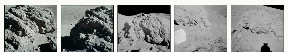
 Top: original Apollo frames. Bottom: Gaussian-splat recoveries of the same views. The splat captures coarse boulder/terrain structure and enough texture contrast to be useful, but it’s visibly incomplete wherever the projected point support is thin.
How good are the synthetic views? (Not very - by design)
Scored against the real photographs, the recoveries are mediocre by image-quality standards:
| Metric | Value |
|---|---|
| Full-image PSNR | 11.26 dB |
| Masked PSNR (covered pixels) | 13.31 dB |
| Mean SSIM | 0.301 |
| Mean mask coverage | 0.543 |
11 dB is nowhere near photo-realistic. But the metric that matters for my use isn’t PSNR - it’s mask coverage: how much of the frame the splat actually supported with projected geometry. Roughly half of each frame is well-supported; the uncovered pixels drag the full-image numbers down. The question isn’t “is this a beautiful render?” It’s “is there enough real local structure here for SfM to find and match features?”
The experiment: N=15 → N=25, and the value of saying no
I generated 10 new camera poses between neighboring recovered cameras, rendered synthetic images there, and formed a 25-image candidate set (15 real + 10 synthetic). Then I re-ran the whole SfM/MVS/mesh pipeline.
Six of the ten synthetic views registered. Four were rejected. And that selectivity is the best part of the result, not a failure of it.
 The ten synthetic novel views. Green borders registered into the augmented SfM run; red borders were rejected. The pattern tracks mask coverage almost perfectly - accepted views averaged 0.622 coverage, rejected ones 0.451.
Think about what happened: SfM acted as an automatic quality gate on my own hallucinations. The high-coverage splats carried enough genuine structure to triangulate consistently and were let in; the sparse, artifact-heavy ones couldn’t find consistent matches and were thrown out. I didn’t have to hand-pick the good synthetic frames - the geometry did it for me. In a domain where generative models cheerfully invent plausible nonsense, a downstream consistency check that refuses the bad inventions is exactly what you want.
What the accepted views actually bought
 Camera coverage, SfM stability, dense-reconstruction gain, and the novel-view fidelity proxy. Six splat views join the 15 originals; sparse and (especially) dense support rise; reprojection error climbs only modestly.
The headline numbers, augmented (N=25) vs. the improved baseline (N=15):
| Metric | N=15 | N=25 | Change |
|---|---|---|---|
| Registered images | 15 | 21 | +6 synthetic |
| Sparse points | 24,704 | 27,807 | +12.6% |
| Mean reprojection error | 0.299 px | 0.340 px | +13.5% |
| Filtered dense points | 382,104 | 565,253 | +47.9% |
| Mesh faces | 2,426,609 | 3,602,301 | +48.4% |
The win is concentrated in the dense stage: nearly 48% more dense points and mesh faces, i.e. substantially more reconstructed surface - for only a small (~0.04 px) rise in reprojection error. And critically, the augmented model didn’t drift: after aligning on the 15 shared camera centers, the symmetric Chamfer distance to the baseline was 0.179% of the bounding-box diagonal, with 99%+ of points in each model lying within 1% of the other.
 Sparse clouds after alignment: photogrammetry-only (N=15) vs. splat-augmented (N=25). Same scene, denser support.
 Robust X-Z projections of mesh vertices. The improved dense path fills more of the terrain volume, and the registered splat views expand surface support further.
The learning, stated plainly: Gaussian splatting helped not by producing reliable new photographs, but by adding intermediate camera support that let the dense stage cover more surface - while staying geometrically faithful to the original scene. More terrain reconstructed, same Moon, slightly noisier cameras. For a hazard or resource map, surface completeness is the thing you’re buying, so that’s a trade worth taking.
Step 2: once you can see the terrain, find the resources
Reconstructing the ground is only half of an off-world prospecting story. The other half is identifying what’s valuable in it - the part of ISRU that turns “here is a rock” into “here is ore.” That’s a separate project of mine, on copper-vein detection, and it’s the natural sequel to the geometry above.
Copper ores like chalcopyrite (CuFeS₂) carry their resource information in vein structure - thin, branching mineralized channels. I attacked this two ways.
(1) The offline 3D pipeline - pixel-accurate vein maps on a mesh. It starts, like the lunar work, from a dense photogrammetric reconstruction - except here the “terrain” is a single chalcopyrite specimen captured under controlled robotic imaging. Here is that actual reconstruction; drag to rotate it, scroll to zoom:
The raw Agisoft reconstruction of the specimen - 74,494 vertices, 148,628 faces, a 2K baked texture (Draco-compressed to ~260 KB for the web). This is the geometry the vein detector actually runs on.
Onto that mesh I fuse three medical-imaging ridge filters (Frangi vesselness, Meijering neuriteness) with color-gated thresholding to find veins in each frame, then project those 2D masks back onto the model through 278-camera consensus voting. The result is a vein map that lives on the 3D surface, with single-view artifacts voted away:
 The same specimen with detected copper veins fused onto the textured mesh via multi-view consensus. This is the “resource map” analog of the lunar terrain mesh.
(2) The real-time 2D scout. The 3D pipeline is accurate but slow - it needs a controlled robotic capture and a full SfM run per specimen. No rover budget survives that for every rock. So I used the Frangi masks as free pseudo-labels to train a Faster R-CNN MobileNetV3-Large FPN detector that runs on plain handheld video:
 Top: input frames. Middle: Frangi pseudo-labels (yellow mask, red boxes) - the auto-generated supervision. Bottom: the trained detector’s predictions. The network reproduces the dominant veins and cleans up the long tail of noisy components.
On a temporally held-out split it reaches a pixel-level F1 of 0.736 (95.0% pixel accuracy) and runs at 6.6 fps on a laptop CPU - with zero human annotation effort.
The trick I’m proudest of: a 1998 medical filter as a free geologist
The Frangi filter was designed in 1998 to enhance retinal blood vessels and neurites. It has nothing to do with rocks. But its inductive bias - thin, elongated, tubular structures of locally consistent width and orientation - is domain-agnostic. Copper veins satisfy exactly that geometric prior. So a medical-imaging ridge filter becomes a zero-cost annotator for geological deep learning: it labels the training data so a human never has to. The Faster R-CNN then learns a smoothed, more conservative version of that prior, gaining robustness to the specular glints that defeat the raw threshold.
That cross-domain borrow is, to me, the most space-relevant idea in the whole project - because off-world you will never have a labeled dataset. You cannot ship 10,000 expert-annotated lunar rock images to a rover. A labeling oracle that needs no humans is not a convenience; it’s a precondition.
Why both halves are really the same lesson
Lunar reconstruction and copper prospecting look unrelated until you notice they’re solving the same constraint from two sides:
- Sparse views → manufacture camera support with splatting, and let geometry reject the bad ones.
- No labels → manufacture supervision with a physics-of-shape filter, and let a CNN smooth it.
- Limited compute → run a cheap real-time scout, and trigger the expensive 3D pipeline only on promising targets.
Every one of those is a do-more-with-less move, and less - fewer images, no labels, less power and comms - is the permanent operating condition of anything autonomous in space. The techniques aren’t just efficient; in the off-world regime they’re often the only option, because the Earth-style fallbacks (go reshoot it, go label more, run it in the cloud) simply don’t exist.
Where I was honest about the limits
- Apollo side: a tiny 15-frame sequence; splat PSNR is low (it’s a scaffold, not a render); reprojection error rose with augmentation; and again - Agisoft beat my hand-built pipeline. The contribution is the augmentation insight, not a new SOTA reconstructor.
- Copper side: a single specimen (cross-ore generalization unverified); the metrics measure agreement with the Frangi prior, not with a human geologist; and the rock is terrestrial chalcopyrite, not lunar regolith. The bridge to actual ISRU is conceptual, not yet demonstrated on planetary material.
Where it goes next
- Train a proper 3D Gaussian-splat (not just geometry-seeded projection) so more synthetic views clear the registration gate.
- Run the augmentation on real orbital / rover imagery (LRO, Chang’e, Perseverance) instead of an Apollo assignment set.
- Add multispectral cues for genuine mineral identification, and gather a small expert-annotated vein test set to escape the pseudo-label ceiling.
Reproduce / dig in
- Real-time copper-vein detector (code, weights, generated labels, rendered video): arjunsinghyadav2/SRAI-copper-vein-fastrcnn
Both projects were solo work for my Robotics & Autonomous Systems studies at Arizona State. The lunar reconstruction was a photogrammetry assignment I pushed into novel-view-augmentation territory; the copper-vein detection grew out of an offline 3D mineral-segmentation pipeline I’d built earlier. Different domains, same obsession: getting 3D understanding out of almost no data.